9  非直角双曲线模型

Thornley (1976) 提出了非直角双曲线模型，它的表达式为：

P_{n} = \frac{\alpha I + P_{nmax} \sqrt{(\alpha I + P_{nmax})^{2} - 4 \theta \alpha I P_{nmax}}}{2 \theta} - R_{d} \tag{9.1}

其中，\theta 为表示曲线弯曲程度的曲角参数，取值为0\leq \theta \leq 1。其他参数意义同式 公式  8.1。同样如同直角双曲线模型，式仍然没有极值，无法求得 I_{sat}，可以仍然参考直角双曲线模型的方式进行计算。

9.1 非直角双曲线模型的实现

library(minpack.lm)

# 读取数据，同fitaci数据格式
lrc <- read.csv("data/lrc.csv")
lrc <- subset(lrc, Obs > 0)

# 光响应曲线没有太多参数，
# 直接调出相应的光强和光合速率
# 方便后面调用
lrc_Q <- lrc$PARi
lrc_A <- lrc$Photo 

# 非直角双曲线模型的拟合
lrcnls <- nlsLM(lrc_A ~ 
                (1/(2*theta))*
                (alpha*lrc_Q+Am-sqrt((alpha*lrc_Q+Am)^2 - 
                4*alpha*theta*Am*lrc_Q))- Rd,
                start=list(Am=(max(lrc_A)-min(lrc_A)),
                alpha=0.05,Rd=-min(lrc_A),theta=1)) 

fitlrc_nrec <- summary(lrcnls)

# 光补偿点
Ic <- function(Ic){
  (1/(2 * fitlrc_nrec$coef[4,1])) * 
    (fitlrc_nrec$coef[2,1] * Ic + fitlrc_nrec$coef[1,1] - 
    sqrt((fitlrc_nrec$coef[2,1] * Ic + fitlrc_nrec$coef[1,1]
    )^2 -  4 * fitlrc_nrec$coef[2,1] * 
    fitlrc_nrec$coef[4,1] * fitlrc_nrec$coef[1,1] * Ic)) -
    fitlrc_nrec$coef[3,1]
}

uniroot(Ic, c(0,50))$root  

[1] 2.234292

# 光饱和点
Isat <- function(Isat){
  (1/(2 * fitlrc_nrec$coef[4,1])) * (fitlrc_nrec$coef[2,1] * 
  Isat + fitlrc_nrec$coef[1,1] - sqrt(
  (fitlrc_nrec$coef[2,1] * Isat +fitlrc_nrec$coef[1,1])^2 - 
  4*fitlrc_nrec$coef[2,1] * fitlrc_nrec$coef[4,1] * 
  fitlrc_nrec$coef[1,1] * Isat)) - 
  fitlrc_nrec$coef[3,1] - (0.9*fitlrc_nrec$coef[1,1])}

uniroot(Isat, c(0,2000))$root

[1] 1596.286

# 使用ggplot2进行作图并拟合曲线
library(ggplot2)
light <- data.frame(lrc_Q = lrc$PARi, lrc_A = lrc$Photo)

nonrec_form <- y ~ 
  (1/(2*theta))*(alpha*x+Am-sqrt((alpha*x+Am)^2 - 
   4*alpha*theta*Am*x))- Rd

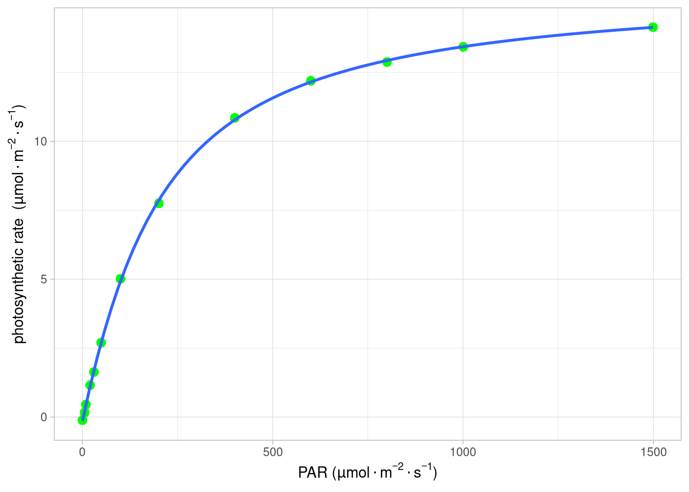
ggplot(light, aes(x = lrc_Q, y = lrc_A)) + 
  geom_point(shape = 16, size = 3, color = "green") + 
  geom_smooth(method="nls", formula = nonrec_form, se = FALSE,
  method.args = list(start = c(Am=(max(lrc_A)-min(lrc_A)), 
  alpha=0.05, Rd=-min(lrc_A), theta=1), 
  aes(color='blue', size = 1.2))) +
  labs(y=expression(paste("photosynthetic rate  ", 
          "(", mu, mol%.%m^-2%.%s^-1, ")")), 
       x=expression(paste("PAR ", 
           "(", mu, mol%.%m^-2%.%s^-1, ")"))) +
  theme_light()

Figure 9.1: 非直角双曲线模型拟合

Table 9.1: 非直角双曲线模型结果

	Estimate	Std. Error	t value	Pr(>|t|)
Am	15.8017296	0.1513064	104.435285	0.0000000
alpha	0.0658067	0.0020216	32.551422	0.0000000
Rd	0.1461717	0.0420800	3.473659	0.0070082
theta	0.3700908	0.0493403	7.500783	0.0000369

最终的数据拟结果如图 Figure 9.1 所示，拟合的参数及结果见表 Table 9.1。单纯从作图来看，本例数据使用非直角双曲线与散点图重合程度更高。

9.2 利用函数来拟合

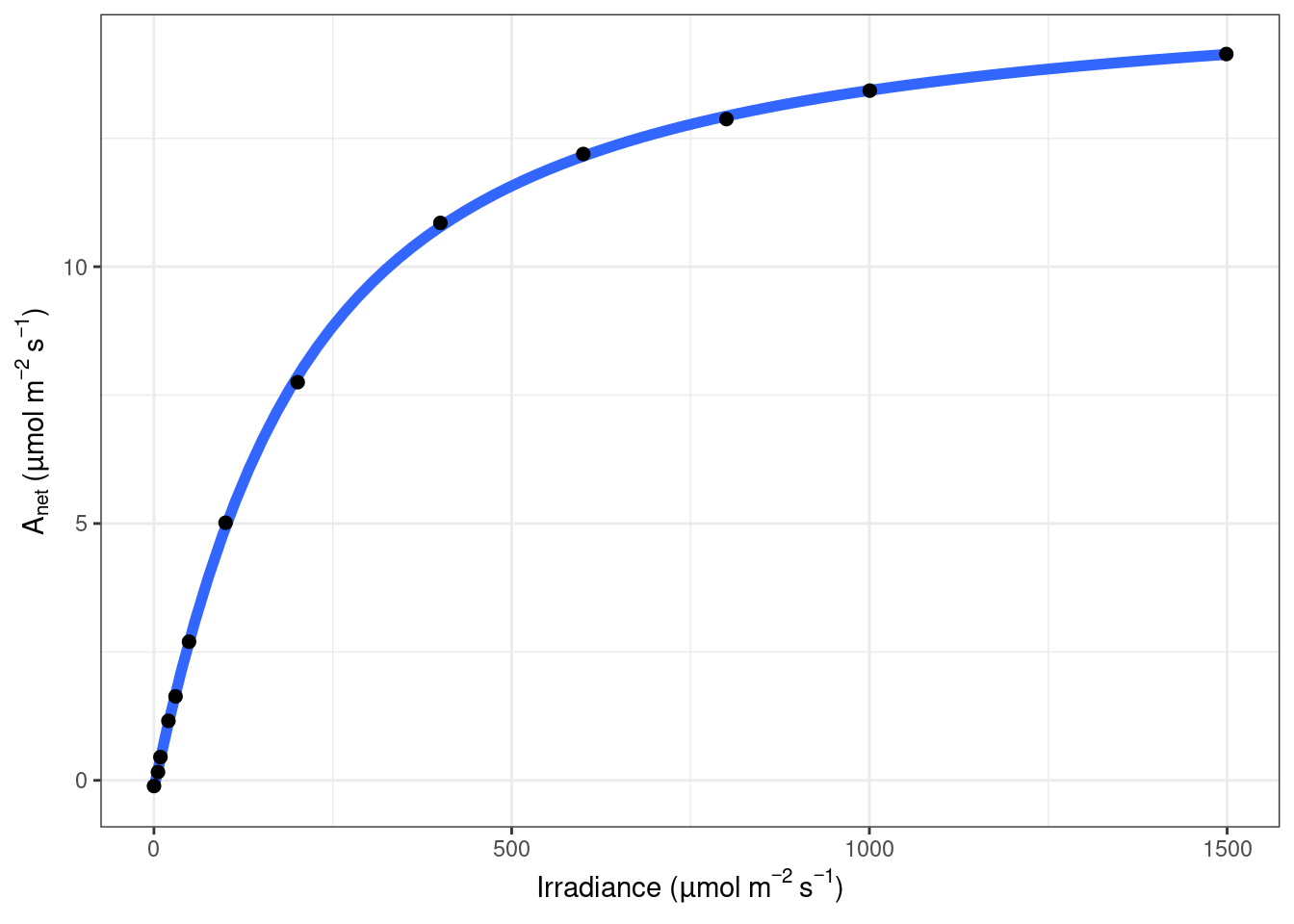
上面的方式是手动实现，也并不复杂，phtosynthesis 和 FitAQ 软件包提供了非直角双曲线模型的相应的函数，可以让我们方便的进行处理。

9.2.1 使用 photosynthesis 处理

安装可以通过 CRAN:

install.packages('photosynthesis')

我们看一下 LI-6400 数据的使用：

library(photosynthesis)
fit6400 <- fit_aq_response(lrc, varnames = list(A_net = "Photo", PPFD = "PARi"))

他的拟合结果的查看方式为：

summary(fit6400[[1]])

Formula: A_net ~ aq_response(k_sat, phi_J, Q_abs = data$Q_abs, theta_J) - 
    Rd

Parameters:
                Estimate Std. Error t value Pr(>|t|)    
k_sat          15.801730   0.151306 104.435 3.43e-15 ***
phi_J.Q_abs     0.065807   0.002022  32.551 1.20e-10 ***
theta_J         0.370091   0.049340   7.501 3.69e-05 ***
Rd.(Intercept)  0.146172   0.042080   3.474  0.00701 ** 
---
Signif. codes:  0 '***' 0.001 '**' 0.01 '*' 0.05 '.' 0.1 ' ' 1

Residual standard error: 0.06845 on 9 degrees of freedom

Number of iterations to convergence: 6 
Achieved convergence tolerance: 1.49e-08

除此以外，它还提供了只看拟合结果的方式：

fit6400[[2]]

         A_sat      phi_J   theta_J        Rd      LCP  resid_SSs
k_sat 15.80173 0.06580668 0.3700908 0.1461717 2.234292 0.04216531

他们的意义按顺序为：

1. 饱和光下的净光合速率 (A_sat)，

2. 表观量子效率 (phi_J),

3. 曲线的弯曲程度 (theta_J),

4. 暗呼吸速率 (Rd),

5. 光补偿点 (LCP),

6. 残差的平方和 (resid_SS)。

也可以直接输出图形，只不过要想定制化，还要自己做：

fit6400[[3]]

photosynthesis 软件包的非直角双曲线拟合图形查看

如果是 LI-6800，稍微修改一下参数即可，这里不再进行一步一步的演示：

aq6800 <- read.csv("data/lrc6800.csv")
fit6800 <-
  fit_aq_response(aq6800, varnames = list(A_net = "A", PPFD = "Qin"))

9.2.2 使用 FitAQ 处理

安装必须是从 github 安装，当然，如果你和我遇到一样登录 github 困难的话，我把他 fork 到 gitee 上去了：

remotes::install_git("https://gitee.com/zhu_jie_dong/FitAQ")
#或
remotes::install_github("MarkusLoew/FitAQ")

使用也比较方便，默认这样操作就行了：

library(FitAQ)
FitAQ(data = lrc, A = Photo, Q = PARi)

         Amax        phi        Rd     theta
Amax 15.80173 0.06580667 0.1461717 0.3700909

如果觉得不满意，还可以手动调整初值，作者考虑的比较周到：

fit1 <- FitAQ(
  data = lrc,
  A = Photo,
  Q = PARi,
  provide.model = TRUE,
  nlscontrol = c(maxiter = 500),
  start = list(
    Amax = 15,
    phi = 0.06,
    Rd = 0.14,
    theta = 0.3
  ),
  lower = c(12, 0, 0, 0),
  upper = c(17, 0.1, 3, 0.5),
  trace = TRUE
)

  0:     2.6244459:  15.0000 0.0600000 0.140000 0.300000
  1:   0.021848654:  15.7837 0.0658725 0.146820 0.377608
  2:   0.021082662:  15.8019 0.0658089 0.146186 0.370045
  3:   0.021082654:  15.8017 0.0658067 0.146172 0.370090
  4:   0.021082654:  15.8017 0.0658067 0.146172 0.370091

summary(fit1)

Formula: A ~ ((phi * Q + Amax - sqrt((phi * Q + Amax)^2 - 4 * theta * 
    phi * Q * Amax)))/(2 * theta) - Rd

Parameters:
       Estimate Std. Error t value Pr(>|t|)    
Amax  15.801729   0.151306 104.435 3.43e-15 ***
phi    0.065807   0.002022  32.551 1.20e-10 ***
Rd     0.146172   0.042080   3.474  0.00701 ** 
theta  0.370091   0.049340   7.501 3.69e-05 ***
---
Signif. codes:  0 '***' 0.001 '**' 0.01 '*' 0.05 '.' 0.1 ' ' 1

Residual standard error: 0.06845 on 9 degrees of freedom

Algorithm "port", convergence message: relative convergence (4)

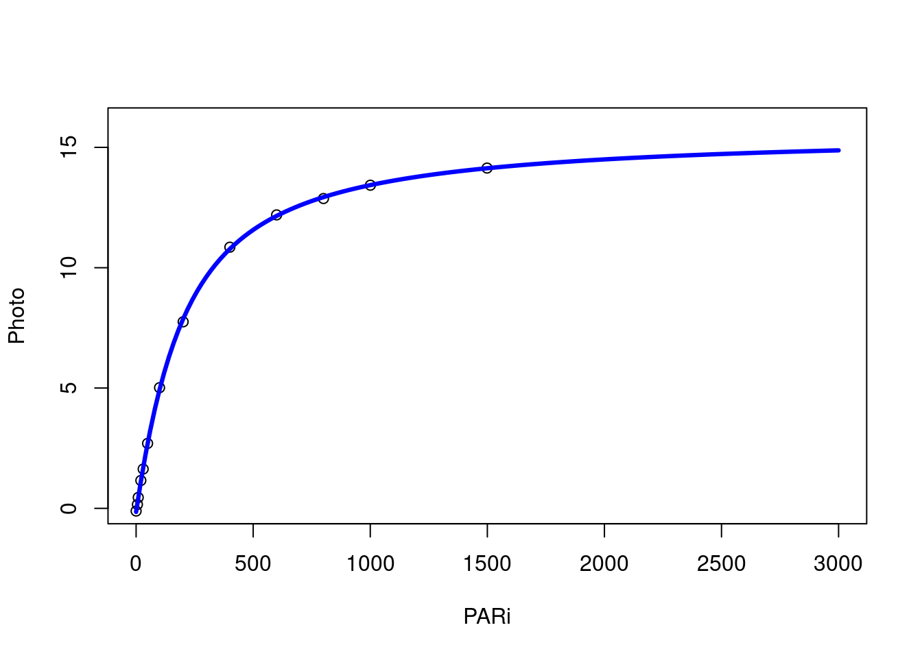
predict_range <- data.frame(Q = seq(from = 0, to = 3000, by = 20))

addline <-
  within(predict_range, A <-
           predict(fit1, newdata = predict_range))
plot(
  Photo ~ PARi,
  data = lrc,
  xlim = c(0, 3000),
  ylim = c(0, 16)
)
lines(A ~ Q, data = addline, col = "blue", lwd = 3.2)

FitAQ 的非直角双曲线拟合

这里需要说明，FitAQ 作者使用的 base R 的语法，而 photosynthesis 则喜欢 ggplot2，这两个谈不上优劣，只是相比而言，photosynthesis 把一些细节都做了，出结果比较省事，但是要做一些定制化图形的时候没有接口，而 FitAQ 则把细节美化留给用户自己来操作，但出基本结果的时候代码量会大一些。定制程度更高一些。

提醒

这里做拟合曲线图形的时候用了一个小技巧，与我 Figure 9.1 所采用的方式完全不同，我的作图实际上是强行把非线性拟合放到 ggplot2 内，而这里不需要拟合过程，只需要参数带入模型，得出数据点来，只要数据点足够密集，我们用线连接所有数据点后，看上去就是一条平滑的曲线，这种方式虽然是欺骗，但是并没有错误，数据点足够密集，我们根本看不出是点还是线来。

饱和点和补偿点的计算也提供了方便的函数：

FitLCP(fit1)

     LCP 
2.234292 

FitSat(fit1)

     LSP 
1455.489 

FitSat(fit1, sat.fac = 0.95, range = c(0, 3200))

     LSP 
2986.574 

饱和点也是使用了达到最大饱和光强多少比例时候的值，带入模型求的光强而得到，例如这里修改后使用了 0.95，看上去结果就不不正常了。

至于 LI-6800 的分析，也是一样，修改光合速率和光合有效辐射两个参数的名称即可：

aq6800 <- read.csv("data/lrc6800.csv")
FitAQ(data = aq6800, A = A, Q = Qin)

         Amax      phi       Rd     theta
Amax 39.05857 0.063463 3.243814 0.7451511

为了减少篇幅，不在展开做过多的介绍，使用方式和上面演示的 LI-6400 一致。

Thornley, J H M. 1976. 《Mathematical models in plant physiology》. London: Academic Press.